City of Helsinki public procurements have been available as open data since 2014. High quality data like this is obviously of great interest to many and [several interesting applications and visualizations] have been made available.
With some additional open data from Finnish Patent and Registration Office and data wrangling, the location of the city supplier companies could be made visible. Geofi-package, just released in CRAN, provides excellent tools for this sort of task, alongside dplyr-package’s lightning-fast join and mutate operations.
The Patent and Registration Office data could be accessed by making API calls with the unique Business ID (“Y-tunnus”) of each company. A limitation was that information was available only for limited companies, cooperatives and similar entities, leaving out public institutions, third sector (independent sector) actors and sole proprietor type enterprises.
Hadley Wickham’s httr-package vignette Best practices for API packages provided a good starting point for building our own custom function “prh_api”, which made it possible to access company information with relative ease. In practice the task was not only smooth sailing as the API had a limit of 300 calls per minute, to be shared between all API users. Downloading information took approximately 4 seconds for one company (15 calls per minute), which added up to a significant amount of hours when the dataset had over 30,000 unique Business IDs.
Downloading and processing the data
Rows with invalid BIDs can be removed with hetu-package’s bid_ctrl-function:
library(hetu)
library(dplyr)
helsingin_ostot <- read.csv("http://openspending.hel.ninja/files/ostot/helsingin-ostot-all.csv")
helsingin_ostot$valid_ytunnus <- bid_ctrl(helsingin_ostot$toimittaja_ytunnus)
helsingin_ostot2 <- helsingin_ostot[which(helsingin_ostot$valid_ytunnus),]
At this point I produced a vector or unique business ID’s from the dataset, so that same information would not be downloaded more than once, and use this dataset to download data from Patent and Registration Office API. However, as the process is so time consuming, I will not reproduce the process. Below is an example with just one Business ID number “0494571-4”:
# A vector containing unique Business IDs
unique_ytunnus <- unique(helsingin_ostot2$toimittaja_ytunnus)

# Example: Getting information for one Business ID and filtering the data

yrityksen_tiedot <- jsonlite::fromJSON("http://avoindata.prh.fi/tr/v1/0494571-4", simplifyVector = TRUE)
poimitut_tiedot <- NULL
poimitut_tiedot$businessId <- yrityksen_tiedot$results$businessId
poimitut_tiedot$street <- yrityksen_tiedot$results$addresses[[1]]$street[1]
poimitut_tiedot$city <- yrityksen_tiedot$results$addresses[[1]]$city[1]
poimitut_tiedot$postCode <- yrityksen_tiedot$results$addresses[[1]]$postCode[1]

poimitut_tiedot <- as.data.frame(poimitut_tiedot)

helsingin_ostot3 <- left_join(x = helsingin_ostot2, y = poimitut_tiedot, by = c("toimittaja_ytunnus" = "businessId"))
With more than one Business ID, the code above can be made into its own function and used with lapply function.
If the company information could be downloaded from the API, the information most likely contained the zip code, address and city of the company. If these are missing it was most likely due to the API call producing error 404. Below is visualized the number of missing zip codes:
# Prepared dataset that has above operations
load("~/helsingin_ostot3.RData")
library(ggplot2)
ggplot(helsingin_ostot3, aes(fill=is.na(postCode), x=year)) +
  geom_bar(position="stack", stat="count") +
  labs(x = "Year", y = "Rows", fill = "Missing \nzip code")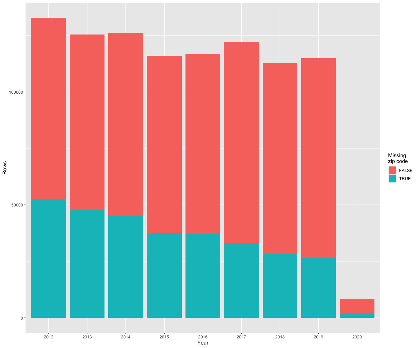
The closer we are to present day, the smaller the proportion of missing data becomes.
Top-20 municipalities with most procurements
Company’s zip code is a good starting point to determine where purchased services, items and materials come from. The data could be visualized with zip code areas, but that would produce a hard to read map with too many details. Municipality level visualization will be adequate for our purposes.
While zip code areas and municipality borders do not always align perfectly, the zip code area can be assigned to the municipality which has the majority of buildings in the zip code area (Tilastokeskus 2020). Keen readers may have noticed that the data from API already had city and even street level data, but as city names can be in Finnish or in Swedish, it is simpler to look up municipality names by using an unambiguous zip code value.
library(geofi)
library(dplyr)
zipcodes <- geofi::get_zipcodes(year = 2021)

# Transform sf-object to a regular data frame
zipcodes <- as.data.frame(zipcodes) %>%
  select(kuntanro, posti_alue)
helsingin_ostot4 <- dplyr::left_join(x = helsingin_ostot3, y = zipcodes, by=c("postCode" = "posti_alue"))

municipalities <- geofi::get_municipalities(year = 2021)
municipalities <- municipalities %>%
  select(kunta, kunta_name)

helsingin_ostot4 <- dplyr::right_join(x = municipalities, y = helsingin_ostot4, by=c("kunta" = "kuntanro"))

# Group procurements by municipality
helsingin_ostot5 <- helsingin_ostot4 %>%
  group_by(kunta_name) %>%
  summarise(kunta_summa = sum(as.numeric(summa), na.rm = FALSE))

# Print top 20 municipalities
slice_max(helsingin_ostot5, order_by = kunta_summa, n = 20)
## Simple feature collection with 20 features and 2 fields (with 1 geometry empty)
## geometry type: MULTIPOLYGON
## dimension: XY
## bbox: xmin: 215353.4 ymin: 6640920 xmax: 588843.4 ymax: 7298654
## projected CRS: ETRS89 / TM35FIN(E,N)
## # A tibble: 20 x 3
## kunta_name kunta_summa geom
## <chr> <dbl> <MULTIPOLYGON [m]>
## 1 <NA> 12164973424. EMPTY
## 2 Helsinki 5214226687. (((402737.7 6680700, 402069.8 6680535, 400326.8 6678…
## 3 Espoo 741586021. (((375773.7 6691597, 377355.9 6680366, 379983.8 6681…
## 4 Vantaa 629136624. (((392811.8 6694857, 399192.7 6692524, 396012.8 6689…
## 5 Kuopio 470253261. (((581015.6 7009317, 585462.3 7007121, 588843.4 7002…
## 6 Kouvola 149758496. (((511075 6780902, 512323 6772856, 508132 6769735, 5…
## 7 Tuusula 129772884. (((397271.6 6711736, 391885.8 6710060, 392411.8 6702…
## 8 Vaasa 90367794. (((259700 7001591, 253892.6 6990776, 242914.5 700120…
## 9 Turku 61425478. (((251038.1 6731422, 245370.1 6713651, 244865.9 6708…
## 10 Tampere 60124288. (((346626.3 6854536, 347270.1 6836030, 334112.1 6814…
## 11 Hyvinkää 51569708. (((396836.4 6726577, 392888.2 6717250, 385516.6 6715…
## 12 Kerava 49833397. (((399192.7 6692524, 392811.8 6694857, 392727.4 6700…
## 13 Raasepori 44527631. (((299881.1 6640940, 297472.1 6640920, 296412.5 6642…
## 14 Oulu 42513844. (((418101.2 7220618, 417351.5 7219858, 415092.4 7219…
## 15 Lahti 42463258. (((448838.6 6774406, 453144.3 6766188, 452204.9 6761…
## 16 Nurmijärvi 22549476. (((385516.6 6715109, 388809.1 6711136, 382590.6 6697…
## 17 Kemi 21518412. (((396561 7287772, 392601.9 7283067, 392361.4 728345…
## 18 Raisio 20195233. (((239031.6 6717088, 236093.7 6712495, 230992.2 6711…
## 19 Porvoo 18877028. (((441843.9 6673817, 440194.5 6673207, 436276.1 6673…
## 20 Padasjoki 18830945. (((422133.8 6800321, 420573.8 6797563, 415159 679860…As expected, the largest sums for procurements were from Helsinki itself and the neighbouring cities of Espoo and Vantaa. Somewhat surprisingly, Kuopio wedges ahead of Kouvola and Tuusula, which are located geographically closer to the Helsinki metropolitan area.
However, the largest amount is credited to the NA group, with 12 billion euros over 8 years. This probably includes for the most part procurements from third sector entities and public sector organizations, highlighting their large role in the Finnish economy.
Choropleth and flow map of the top 20 municipalities
library(sf)
library(dplyr)

# Remove NA group
helsingin_ostot6 <- helsingin_ostot5 %>%
  filter(kunta_name %in% setdiff(helsingin_ostot5$kunta_name, c(NA)))

kunnat_top20_summat <- slice_max(helsingin_ostot6, order_by = kunta_summa, n = 20)

# Highlighting the top 20 with red borders
ggplot() +
  geom_sf(data = helsingin_ostot6, aes(fill = kunta_summa), color = alpha("white", 1/3)) +
  labs(fill = "Helsingin ostot, €") +
  scale_fill_gradient2(n.breaks = 6, trans = "log10") +
  geom_sf(data = kunnat_top20_summat, col="red", size=1)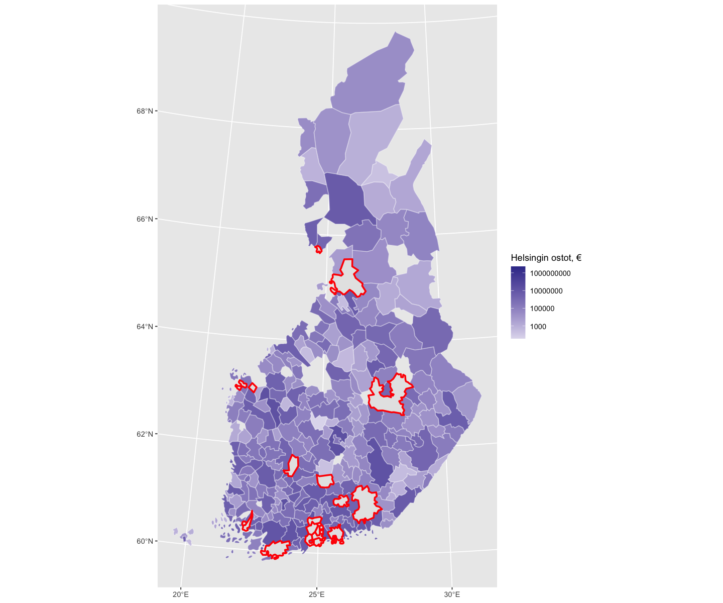
Geofi-package has the option to draw municipality central localities as POINT-geometries. With small modification these can be turned into LINESTRINGs, which have a starting point at the municipality and end point in Helsinki, that can be thought of as flow markers. The example below is very rudimentary, but at their best flow maps can be very beautiful and convey information in fresh and elegant ways.
keskukset <- geofi::municipality_central_localities

# Turn ALL CAPS municipality names to Capital Case with custom capwords-function found in base R
capwords <- function(s, strict = FALSE) {
    cap <- function(s) paste(toupper(substring(s, 1, 1)),
                  {s <- substring(s, 2); if(strict) tolower(s) else s},
                             sep = "", collapse = " " )
    sapply(strsplit(s, split = " "), cap, USE.NAMES = !is.null(names(s)))
}

keskukset$teksti <- capwords(keskukset$teksti, strict = TRUE)

keskukset <- left_join(keskukset, as.data.frame(helsingin_ostot6)[,1:2], by = c("teksti" = "kunta_name"))

# Count the distance between municipalities and Helsinki for later use
keskukset$distance_to_hel <- NULL
keskukset$distance_to_hel <- st_distance(keskukset$geom, y=keskukset$geom[210,])
keskukset$distance_to_hel <- as.integer(keskukset$distance_to_hel / 1000)

# Make linestrings
keskukset_linestring <- st_cast(st_union(keskukset$geom[1,], keskukset$geom[210,], by_feature=TRUE),"LINESTRING")
for (i in 1:nrow(keskukset)) {
  keskukset_linestring[i] <- st_cast(st_union(keskukset$geom[i,], keskukset$geom[210,], by_feature=TRUE),"LINESTRING")
}

keskukset_helsinkiin <- keskukset

keskukset_helsinkiin$geom <- keskukset_linestring

keskukset_helsinkiin <- keskukset_helsinkiin[which(keskukset_helsinkiin$teksti %in% kunnat_top20_summat$kunta_name),]

# Line thickness: 0 for Helsinki, Espoo and Vantaa, and then 4,3,2,2,1...
ggplot() +
  geom_sf(data = helsingin_ostot6, aes(fill = kunta_summa), color = alpha("white", 1/3)) +
  labs(fill = "Helsingin ostot, €") +
  scale_fill_gradient2(n.breaks = 6, trans = "log10") +
  geom_sf(data = arrange(keskukset_helsinkiin, desc(kunta_summa)), col=alpha("red", 1/2), size=c(0,0,0,4,3,2,2,rep(1, 13)))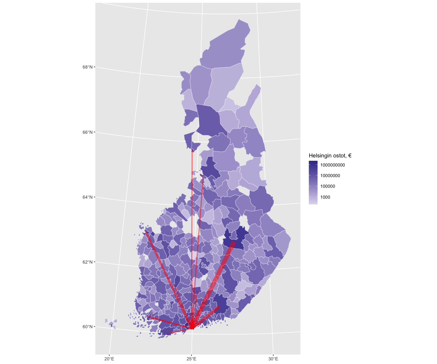
For the above example to work, it is important to keep the desired data object in the class “sf” so that ggplot2 can find geom column without trouble.
Effect of distance and number of companies in a municipality
Finally, I will illustrate how the number of companies in a municipality and municipality’s distance from Helsinki affect how much city of Helsinki buys from there.
library(sf)

# Get number of companies in each municipality from Statfin
# /PXWeb/api/v1/fi/StatFin/yri/alyr/statfin_alyr_pxt_11dc.px
library(pxweb)
library(fuzzyjoin)

pxweb_query_list <-
  list("Vuosi"=c("2019"),
       "Kunta"=c("*"),
       "Tiedot"=c("Tplukumaara2"))

# Download data
px_data <-
  pxweb_get(url = "https://pxnet2.stat.fi/PXWeb/api/v1/fi/StatFin/yri/alyr/statfin_alyr_pxt_11dc.px",
            query = pxweb_query_list)

# Convert to data.frame
px_data_frame <- as.data.frame(px_data, column.name.type = "text", variable.value.type = "text")

yritykset <- left_join(x = px_data_frame, y = as.data.frame(helsingin_ostot5), by=c("Kunta"="kunta_name"))

# Remove "KOKO SUOMI", "Tuntematon" (Unknown) ja municipalities that had no procurements from Helsinki
yritykset <- yritykset[which(!is.na(yritykset$kunta_summa)),]
# Remove geom-column
yritykset <- as.data.frame(yritykset)
yritykset <- yritykset[,-5]

keskukset <- geofi::municipality_central_localities

keskukset <- left_join(keskukset, as.data.frame(helsingin_ostot6)[,1:2], by = c("teksti" = "kunta_name"))

keskukset$distance_to_hel <- NULL
keskukset$distance_to_hel <- st_distance(keskukset$geom, y=keskukset$geom[210,])
keskukset$distance_to_hel <- as.integer(keskukset$distance_to_hel / 1000)

keskukset <- keskukset %>%
  dplyr::select(teksti, distance_to_hel, geom)

# Fuzzyjoin-package removes the need for custom functions
yritykset <- fuzzyjoin::regex_left_join(x = yritykset, y = keskukset, by=c("Kunta" = "teksti"), ignore_case = TRUE)

# Remove outlier, Helsinki
yritykset <- yritykset[-which(yritykset$Kunta == "Helsinki"),]

# Draw scatter-plots with smoothened curves
par(mfrow=c(1,2))
scatter.smooth(x=yritykset$`Yritysten toimipaikat (lkm)`, y=log10(yritykset$kunta_summa), span = 1/5)
scatter.smooth(x=yritykset$distance_to_hel, y=log10(yritykset$kunta_summa))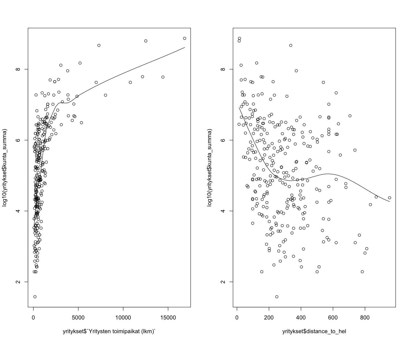
# Compare two different regression models
fit1 <- lm(log10(kunta_summa) ~ `Yritysten toimipaikat (lkm)`, data=yritykset)
fit2 <- lm(log10(kunta_summa) ~ `Yritysten toimipaikat (lkm)` + distance_to_hel, data=yritykset)

# If needed, draw regression plots
# abline(lm(log10(kunta_summa) ~ `Yritysten toimipaikat (lkm)`, data=yritykset))
# abline(lm(log10(kunta_summa) ~ `Yritysten toimipaikat (lkm)` + distance_to_hel, data=yritykset))

summary(fit1)
##
## Call:
## lm(formula = log10(kunta_summa) ~ `Yritysten toimipaikat (lkm)`,
## data = yritykset)
##
## Residuals:
## Min 1Q Median 3Q Max
## -3.2431 -0.7991 0.0834 0.9631 2.4039
##
## Coefficients:
## Estimate Std. Error t value Pr(>|t|)
## (Intercept) 4.75557723 0.07845464 60.62 <0.0000000000000002
## `Yritysten toimipaikat (lkm)` 0.00039387 0.00003411 11.55 <0.0000000000000002
##
## (Intercept) ***
## `Yritysten toimipaikat (lkm)` ***
## ---
## Signif. codes: 0 '***' 0.001 '**' 0.01 '*' 0.05 '.' 0.1 ' ' 1
##
## Residual standard error: 1.159 on 294 degrees of freedom
## Multiple R-squared: 0.312, Adjusted R-squared: 0.3097
## F-statistic: 133.3 on 1 and 294 DF, p-value: < 0.00000000000000022summary(fit2)##
## Call:
## lm(formula = log10(kunta_summa) ~ `Yritysten toimipaikat (lkm)` +
## distance_to_hel, data = yritykset)
##
## Residuals:
## Min 1Q Median 3Q Max
## -3.3314 -0.7943 0.1029 0.9196 2.7113
##
## Coefficients:
## Estimate Std. Error t value
## (Intercept) 5.24186205 0.13519748 38.772
## `Yritysten toimipaikat (lkm)` 0.00036832 0.00003366 10.943
## distance_to_hel -0.00158104 0.00036166 -4.372
## Pr(>|t|)
## (Intercept) < 0.0000000000000002 ***
## `Yritysten toimipaikat (lkm)` < 0.0000000000000002 ***
## distance_to_hel 0.0000172 ***
## ---
## Signif. codes: 0 '***' 0.001 '**' 0.01 '*' 0.05 '.' 0.1 ' ' 1
##
## Residual standard error: 1.126 on 292 degrees of freedom
## (1 observation deleted due to missingness)
## Multiple R-squared: 0.3543, Adjusted R-squared: 0.3499
## F-statistic: 80.13 on 2 and 292 DF, p-value: < 0.00000000000000022We notice that the number of companies in a municipality and distance from Helsinki are significantly correlated with how successful companies from these municipalities are in selling goods and services to Helsinki. There are, however, some interesting outliers in smaller municipalities that punch above their weight in Helsinki’s procurements. The dataset provides an excellent starting point in identifying these companies and, perhaps, learning from their example.
Conclusion
Many of the largest companies in Finland have their headquarters in the capital region (cf. Manninen & Tölli 2019), which may explain why Helsinki, Espoo and Vantaa are so well represented in Helsinki’s procurements. It might be interesting to compare in the future whether regional capitals such as Turku and Tampere also buy majority of their goods and services from the capital region or if they have their own local ecosystems.
Idealized conditions of perfect competition (no barriers to entry or exist, perfect information, zero transaction costs etc.) do not exist even within a relatively homogeneous national framework, let alone within a heterogeneous single market area such as the EU. For different industry advocacy groups, government organizations and companies support for greater access to EU single market offers great potential and active policy measures aim to lower those barriers to entry to foster competitiveness. Perhaps there is still work left undone in opening up access to local markets such as Helsinki.