Probabilistic programming approach for regional trends in apartment prices
Basing on open data from Statistics Finland, we at Reaktor modelled Finnish apartment prices and their trends on zip-code level, in the years 2005–2014. Estimates from the model are available as an interactive visualization.
Why do (statistical) modeling?
The original price data consists of local (geometric) mean sales prices per year. The number of sales is available as well. If there are less than six sales, the mean price is censored.
Partly missing data and noise from low number of transactions make it hard to evaluate local price levels, let alone their changes, except on the most urban areas.
Yearly numbers of transactions for a few random zip codes are depicted on the left below. Censored slots are with red. On the right, all year-zip slots are ordered on the x-axis by their available number of sales data. 17.5% of slots are censored, and about half of the mean prices are either missing or based on less than 30 transactions.
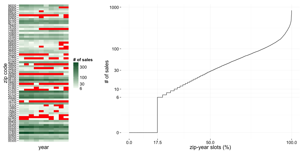
Mean price of 6–30 sales is not a reliable estimate of the local mean, and deriving trends from so few sales is not going to be successful. (Still, it is repeatedly tried: There have been several top and bottom lists of apartment prices and their development published in the Finnish media lately. The media estimates are based on this raw data.)
A statistical model has a concept of a price level behind individual sales. It can then make a distinction between systematic variation of the underlying price level over time and place, and random variation that is not explainable within the model. This is in contrast to looking at raw data without a model; then all variation is taken at face value.
When the model is estimated, it produces the underlying price level as its output. Of course, because the model cannot explain all variation in data, the price level estimates will also have a random component: Instead of a fixed value, we get a probability distribution. Means, trends, confidence intervals, etc., can be computed from these posterior distributions. Provided the model is sensible, these estimates of underlying price trends are more informative than the raw data. Uncertainty of the estimates also reveals when data is not enough to draw any conclusions.
Some properties of zip code areas, like population density, will correlate strongly with apartment prices. Such properties, if known and included in the model, allow us to generalize over zip codes: estimates of price level become available even on places where the data is sparse or there is no data at all. Of course, uncertainty will then be higher, and the model will tell us that.
Adjacency of the areas, or their hierarchy, can be used in the similar way to allow generalization between close-by areas. Once topography or hierarchy is parameterized to the model, it can see correlations between areas that are close to each other, or within the same larger area in the hierarchy. It will then generalize over areas, which helps especially when an area has few observations by itself.
Note that as with demogrpahic covariates, no strict assumptions about geographic dependency are coded into the model. Rather, including these auxiliary parts allows the model to use dependency where it exists.
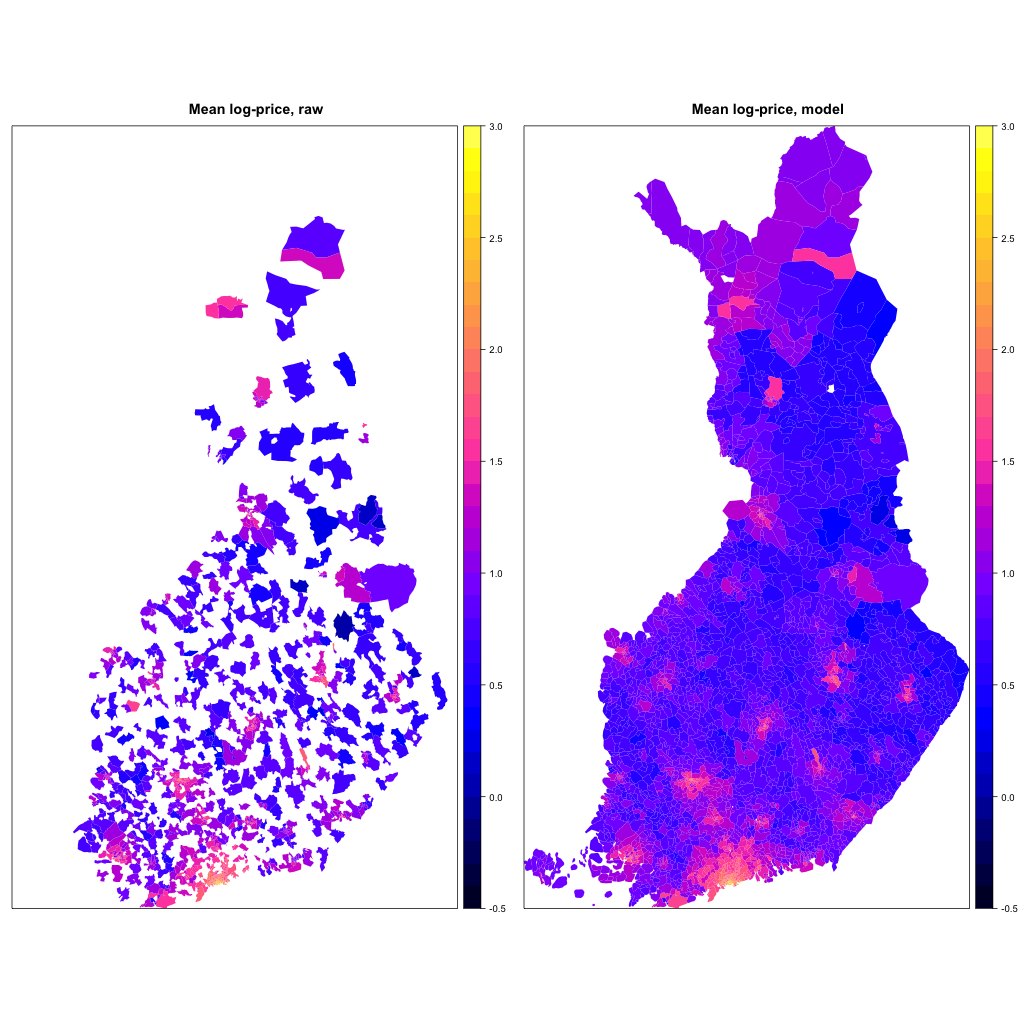
Below, the map on the left shows raw mean prices over the whole period 2005–2014. White areas are without any available data. Map on the right shows the (mean) price level estimated from a model.
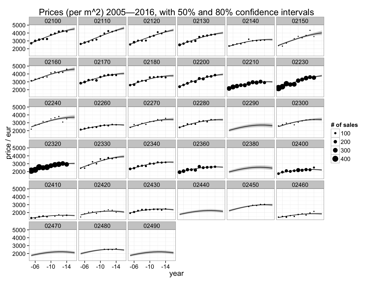
Below, yearly mean prices and estimates of the underlying price level are depicted for some zip codes at Espoo, part of the capital area of Finland. Shading around the lines indicate uncertainty of the estimates. Even within this relatively urban region, estimates from some areas are quite noisy: 02150 or Otaniemi, 02240 or Friisilä, 02330 or Kattilalaakso, etc. Some areas have no sales at all. (But they may not have apartments either. The model does not know whether apartments exist.)
The model can be used for forecasting, but future prices or trends will have large uncertainty, even larger than indicated by the model. The current model has quadratic shape for the temporal dependency. It was chosen to fit the data of the last decade and to give an idea of past price development that is easy to summarise. There is no reason why future changes in economy and policy would follow the same pattern. Althought relative development of areas is more accurately predicted than absolute price levels or trends, the model is at its best at describing past development of apartment prices, especially their spatial differences. There is no guarantee future will follow the same pattern.
The model, data, and environment are described in more detail below.
Environment and data
We used R for almost all data manipulation, modeling and visualizations. Model itself was estimated with Stan. Source code for the project, except for the web site, is available in our GitHub repo.
The libraries pxweb and gisfin make it easy to get apartment prices and other data from the public API’s. The libraries are developed in the Louhos and Ropengov projects. Zip code areas are from Duukkis. Scripts used for downloading data and manipulating it are available in our repo.
Map
Zip code polygons are available at least through the Paavo API and from Duukkis. Finland’s archipelago is extensive and complex, so zip codes extend well onto the Baltic sea. Paavo offers two versions of the polygons, with or without the sea area. The zip code areas with sea can be intersected with the sea shore line, giving us a quite beautiful Finnish zip code map. The problem is its size: over 20MB in the GeoJSON format. We ended up using the polygons from Duukkis: They are a good compromise between size and accuracy.
The set of zip codes varied a little bit from source to source, so some zip codes areas may be missing from the visualizations. A few small areas have no population, or the information about population is missing. These polygons are without a price estimate and appear as grey on the maps.
Note that the model produces price and trend estimates even for areas with no apartments: just the relative position of the zip code and the local population density are enough for computing the estimate.
Model
Of the past sales, the model has yearly (geometric) average per location, and the associated number of sales, if these are not censored ($n<6$). The latter scales the variance of the mean as an estimator of the population mean. Population mean is here the hypothetical mean of all potential apartment sales on the areas. Of course all apartments are not sold at the same rate, so mean is biased towards prices of the apartments that are sold more often.
Sparseness of the data is a problem especially for estimates of temporal price changes, and also for comparison of areas. Predictive covariates for the zip code areas are therefore valuable. A quite extensive set of demographic variables is available in the Paavo data, but of these the model so far has only the population density included. It is probably the most predictive of the covariates, although not necessarily causal from the economics point of view.
Spatial structure is included as a zip code prefix hierarchy. For example 02940 is within the Uusima district (0), city of Espoo (02), and northern Espoo (029). The hierarchy allows the model to see similarity within these and other equivalent nested areas. Real spatial continuity in the form of a Markov field or a latent gaussian field would be an alternative, but it would be much harder to estimate with the chosen tools, and may not be better on modelling administrative areas that are nested, after all.
Temporal change of prices is as interesting as their overall level. The model could have a separate price level for each year, but continuity over time would then be lost, and there would be no predictions. Also the relationships between price trends and covariates (population density) and between trends and spatial or hierarchical structure would be hard to define, for there would be no unique trend. These reasons and simplicity favor a simple temporal parameterization, as the current quadratic model. Combining hierarchy and covariates with a more flexible temporal model, like a gaussian process, is an interesting research question.
In total, there are three parameters on the zip code level affecting log-scale prices: price level, its trend, and change of trend. On the next geographic hierarchy level three other parameters appear: the influences of (logarithmic) population density on price, trend and its change. These six parameters, three plus their interactions with population density, appear also on upper hierarchy levels. On each hierarchy level, the model has multinormal priors for the three or six parameters, and hyperpriors for the variance and covariance of the multinormal distribution. The covariances bind different parameters together, so that for example price level helps the estimation of price trend, or the influence of population density.
In summary, the lowest level of the model for the log prices is
$$ \log h_{it} = \beta_{i1} + \beta_{i2} t + \beta_{i3} t^2 + \beta_{i’4} d_i + \beta_{i’5} d_i t + \beta_{i’6} d_i t^2 , $$
$$ \log y_{it} \sim \textrm{t}\ \left(\log h_{it}, \sqrt{\sigma^2_y + \frac{\sigma^2_w}{n_{it}}}, \nu\right) , $$
where $i$ refers to the zip code area, $t$ is time, $\beta$ are coefficients specific to the zip code $i$, $i’$ is the first prefix hierarchy level of the zip code (population density parameters are constant within each $i’$-area), $t()$ is the t-distribution, $\sigma_y$ is standard deviation of the underlying (log) price levels over years, $\sigma_w$ standar deviation of the prices within the measurement unit (year $\times$ zip), and $\nu$ the degrees of freedom of the residual t-distribution. Note that the linear model is for log-scale prices. The complete model is best described by the source code. Estimate for $\nu$ is around 6.5, that is, residuals are with a bit heavier tails than normal. From the covariance parameters (Omega in the source) one sees that price level and trend correlate at the lowest level ($r$=0,28), as do trend change and price level ($r$=0,43). So price differences between areas have been growing during the last ten years, probably due to urbanisation, a global trend.
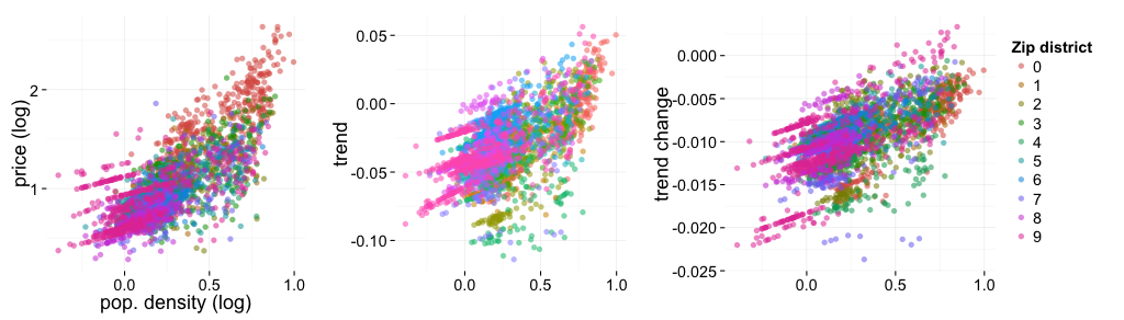
Plotting area-wise prices and its changes against population density, one sees the expected correlation: remote areas are loosing in the sense of price, trend and trend change.
The model has been written and estimated with the probabilistic programming language Stan (http://mc-stan.org/). Stan produces a Monte Carlo estimation algorithm from a generative model description.
Possible improvements
The model could have more demographic covariates. Dealers have reminded us about the predictivity of the sales volume. Obviously, the number of sales is not in a predictive role in the current model.
Apartment vary by their size, age, etc., but this heterogeneity is not taken into account. Trends are biased towards apartments that are sold more often. Some public data is available where sales are separated by size and age of the condos, but these data are even more sparse than the aggregate data used here.
On the Finnish equivalent of this blog, Herra Huu suggested whitened parameterization, which may help with estimation.