We have slowly started developing a follow-up package with ropengov-posse for gisfin-package named geofi. Package provides access to few sources of Finnish open geospatial data from R. We are focusing in administrative regions at the moment and our primary source of data is Statistics Finland and their wfs-api. You can use functions in geofi fecth data such as municipality borders, postal code areas sekä population grids.

geofi is not published in CRAN yet and you cant install it using install.packages(). But you can install it directly from Github with remotes::install_github("ropengov/geofi") and try out the following examples. For quick access try our Shiny app at: https://muuankarski.shinyapps.io/geofi_selain/.

Municipalility borders

library(geofi)
library(ggplot2)

municipalities <- get_municipalities(year = 2020, scale = 4500)
ggplot(municipalities) + 
  geom_sf(aes(fill = as.integer(kunta))) +
  scale_fill_viridis_c()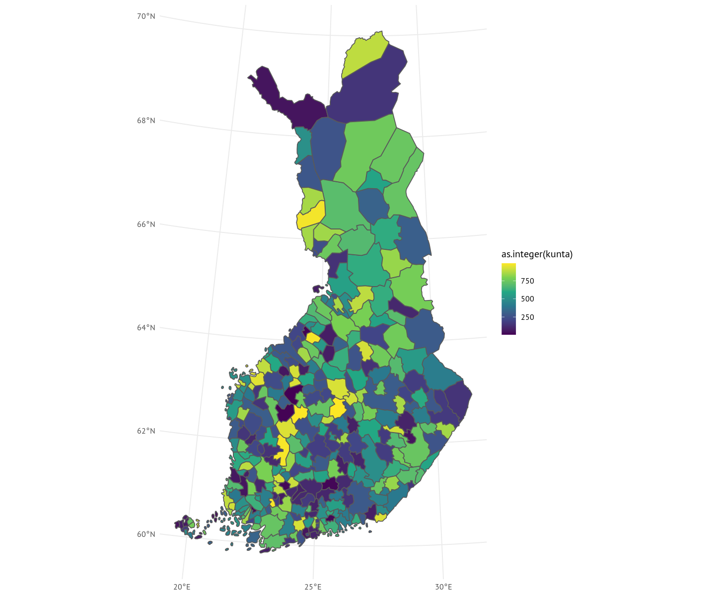

Postal code areas

zipcodes <- get_zipcodes(year = 2020) 
ggplot(zipcodes) + 
  geom_sf(aes(fill = as.integer(posti_alue)), color = alpha("white", 1/3)) +
  scale_fill_viridis_c()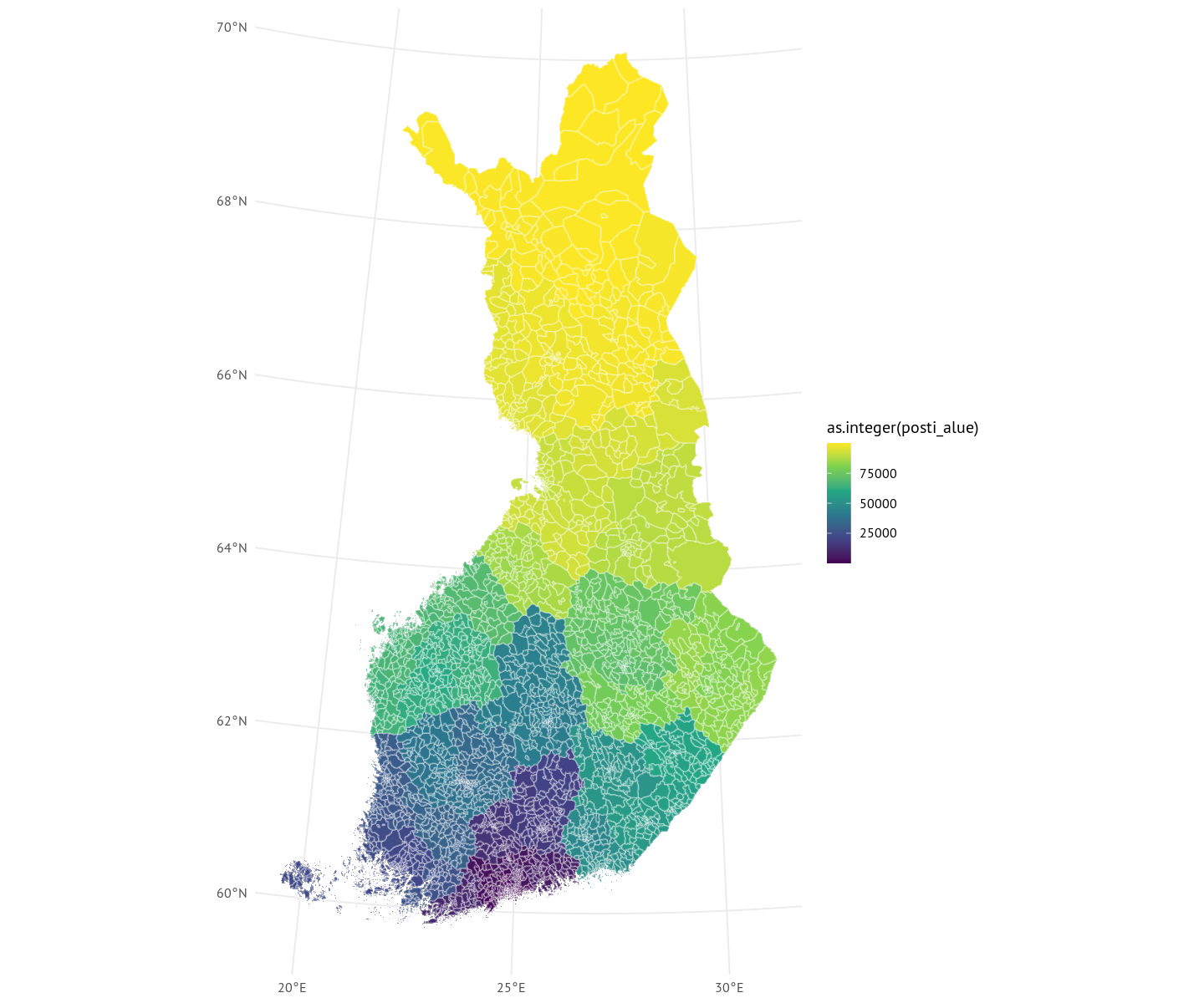

Population grids

pop_grid <- get_population_grid(year = 2018, resolution = 5)
ggplot(pop_grid) + 
  geom_sf(aes(fill = objectid), color = alpha("white", 1/3)) +
  scale_fill_viridis_c()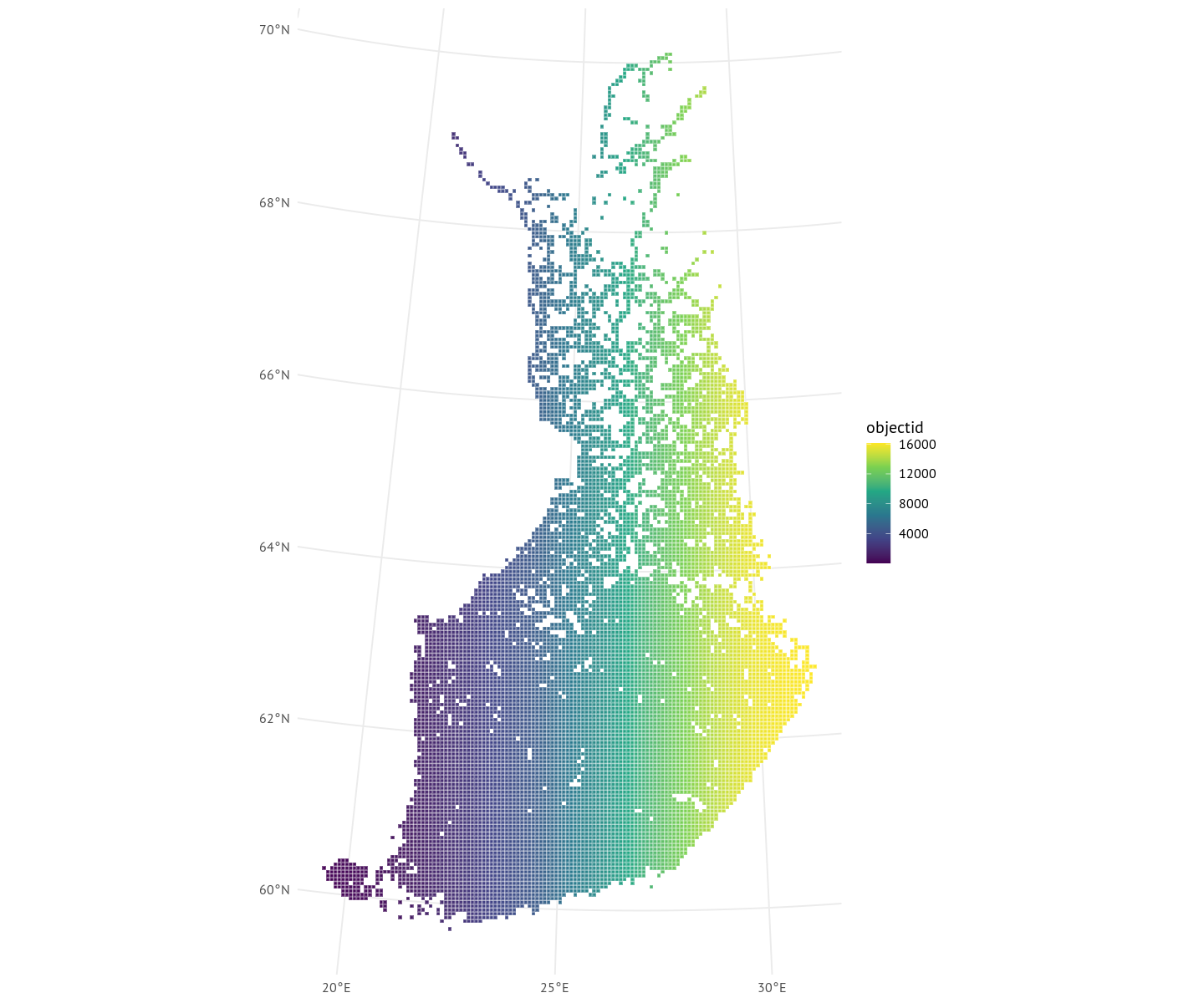

Regions (maakunnant), health care districts (sairaanhoitopiirit) and many more regional breakdowns are based on municipality divide. get_municipalities()-function returns data containing these attribute variables (year 2020), that you can use to aggregate from municipality level upwards.

library(dplyr)
municipalities <- get_municipalities(year = 2019, scale = 4500)
regions <- municipalities %>% 
  group_by(maakunta_name_fi) %>% summarise()
ggplot(regions) + 
  geom_sf(aes(fill = maakunta_name_fi)) +
  scale_fill_viridis_d()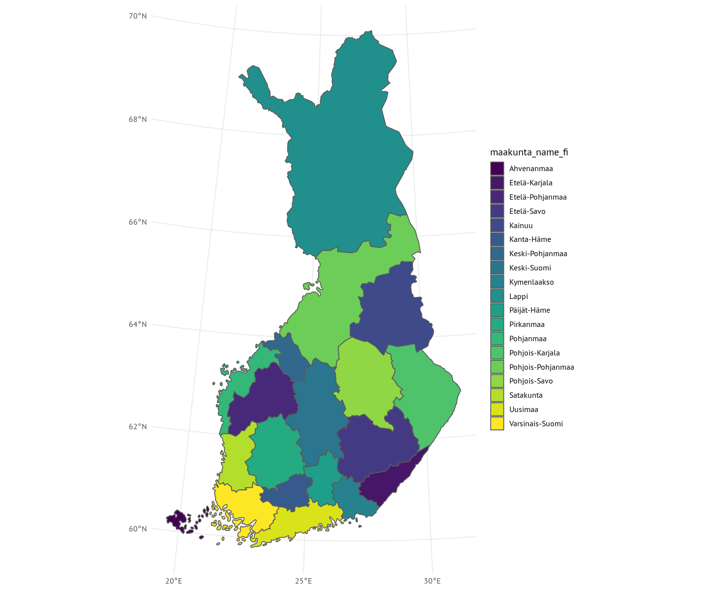

You can join geofi datas with other attribute, too. Below is an example on how to get (non-spatial statistical) data from Statistics Finland and create a map on population at municipality level.

library(tidyr)
library(pxweb)
library(janitor)

municipalities17 <- get_municipalities(year = 2017)

# pull municipality data from Statistics Finland
pxweb_query_list <-
  list("Alue 2019"=c("*"),
       "Tiedot"=c("*"),
       "Vuosi"=c("2017"))
px_data <-
  pxweb_get(url = "http://pxnet2.stat.fi/PXWeb/api/v1/fi/Kuntien_avainluvut/2019/kuntien_avainluvut_2019_aikasarja.px",
            query = pxweb_query_list)
# Convert to data.frame
tk_data <- as.data.frame(px_data, column.name.type = "text", variable.value.type = "text")
tk_data2 <- tk_data %>%
  rename(name = `Alue 2019`) %>%
  mutate(name = as.character(name),
         # Paste Tiedot and Vuosi
         Tiedot = paste(Tiedot, Vuosi)) %>%
  select(-Vuosi) %>%
  spread(Tiedot, `Kuntien avainluvut`) %>%
  as_tibble()
tk_data3 <- janitor::clean_names(tk_data2)

# Join with Statistics Finland attribute data
dat <- left_join(municipalities17, tk_data3)

ggplot(dat) + 
  geom_sf(aes(fill = vakiluku_2017), color = alpha("white", 1/3)) +
  scale_fill_viridis_c(trans = "sqrt")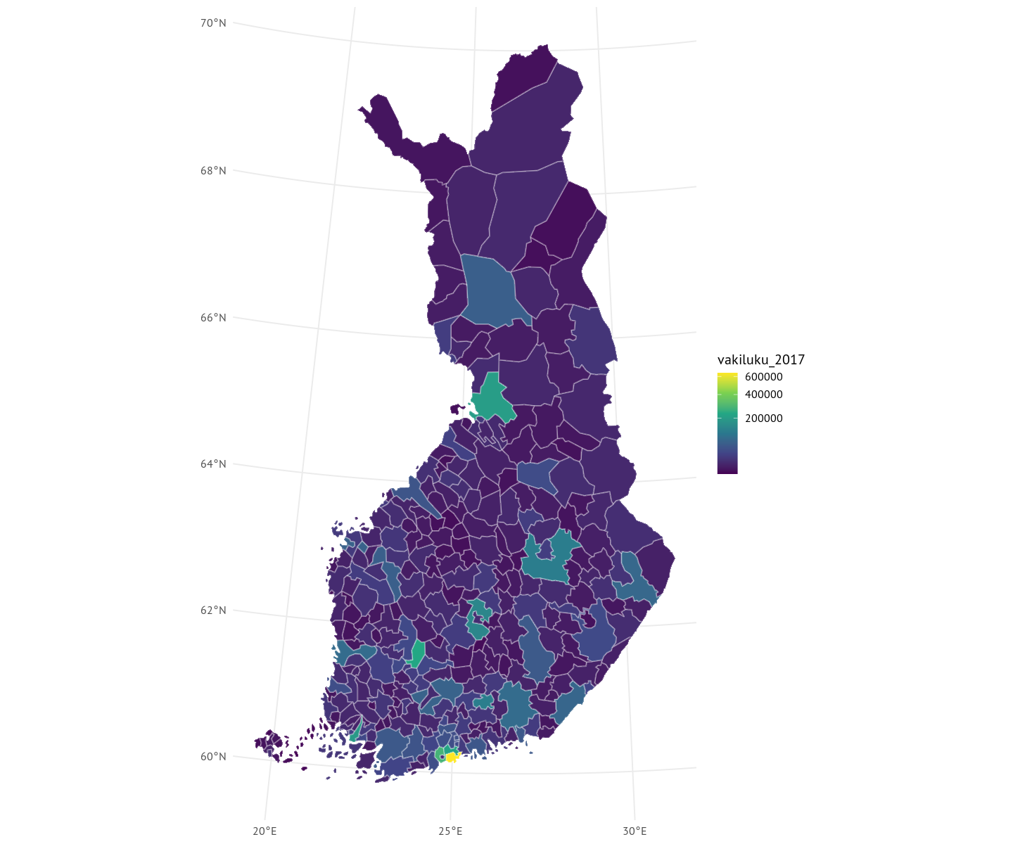

Take a look at the Github-site and join us!